Database tips and tricks

Having worked with databases for 9 years, I have collected some tips and tricks that help me design and operate database systems more effectively and easily. In this post, I will list them and explain why they are so useful.

Timestamp vs boolean flag column

We are all familiar with the design choice of using a flag column, for example, a boolean column to indicate whether a record is active or not. However, this approach can lead to some limitations, such as difficulty in tracking changes over time or querying historical data. Instead, consider using a timestamp column to indicate when a record was created or modified. This allows for more flexibility in querying and can provide valuable context for understanding the state of the data at any given point in time.

So, to demonstrate my points, let’s examine some examples below and see which gives you more information:

Purpose	Boolean Column	Timestamp column
Active Or Inactive?	is_active = true/false	activated_at = null/2025-08-24T07:44:48.071Z
Deleted or not?	is_deleted = true/false	deleted_at = null/2025-08-24T07:44:48.071Z

Definitely, the timestamp column provides more information and context about the state of the data over time. Furthermore, it works very well with indexes, which helps you a lot in querying and optimizing performance.

But, what does it cost us? Let’s test it with these configurations:

-- PostgreSQL
-- Create two tables 

CREATE TABLE with_boolean (
    id SERIAL PRIMARY KEY,
    is_active BOOLEAN NOT NULL DEFAULT TRUE
);

CREATE TABLE with_timestamp (
    id SERIAL PRIMARY KEY,
    activated_at TIMESTAMP NOT NULL DEFAULT CURRENT_TIMESTAMP
);

-- Check table size, both show 8192 bytes
SELECT pg_total_relation_size('with_boolean') as with_boolean_size, 
    pg_total_relation_size('with_timestamp') as with_timestamp_size;

-- Then insert 1 million rows into each table
INSERT INTO with_boolean (is_active) SELECT (i % 2 = 0) FROM generate_series(1, 1000000) AS s(i);
INSERT INTO with_timestamp (activated_at) SELECT (CURRENT_TIMESTAMP - (i * interval '1 second')) FROM generate_series(1, 1000000) AS s(i);

-- Make sure we flush all buffers to disk
CHECKPOINT;
-- Refresh analytics
ANALYZE with_boolean;
ANALYZE with_timestamp;

-- Run table size checking again
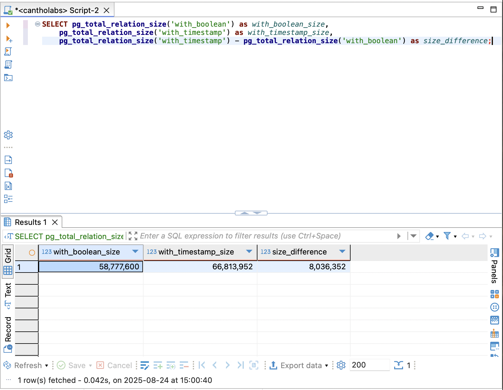
SELECT pg_total_relation_size('with_boolean') as with_boolean_size, 
    pg_total_relation_size('with_timestamp') as with_timestamp_size,
    pg_total_relation_size('with_timestamp') - pg_total_relation_size('with_boolean') as size_difference;

And you know what? They show different sizes at ~8MB for 1 million rows. For me, it’s a good trade-off to obtain better information.

Make your ID column cluster naturally

Why would you choose auto-incrementing IDs or UUID v4 when you have a better choice? Look at my article The ID chosen to get more details on why you should use Lexicographically Sortable Identifiers (LSIDs) like ULID or UUID v7.

The most beneficial aspect of using LSIDs is that they are naturally ordered, which can improve query performance and reduce fragmentation. This is especially important for large tables that you often do time-range queries on. For example, a transaction table in a finance system or a webhook event table in an event-driven architecture.

In PostgreSQL, the primary key is not automatically a clustering index. You need to use the CLUSTER command to physically reorder the table data.

Let’s use combined indices

Let’s start with this setup

-- PostgreSQL
-- Create two tables: user_single_index and user_combine_indices

CREATE TABLE user_single_index (
    id SERIAL PRIMARY KEY,
    name TEXT NOT NULL,
    age INT NOT NULL,
    city TEXT NOT NULL
);

CREATE TABLE user_combine_indices (
    id SERIAL PRIMARY KEY,
    name TEXT NOT NULL,
    age INT NOT NULL,
    city TEXT NOT NULL
);

-- Insert 1 million row into user_single_index
INSERT INTO user_single_index (name, age, city)
SELECT 
    CASE WHEN i % 1000 = 0 THEN 'Alice' ELSE LEFT(repeat(gen_random_uuid()::text, 36), 256) END, -- only ~0.1% are Alice, others get a random 256-char string
    (i % 80) + 18,                                       -- age 18-97
    CASE WHEN i % 5000 = 0 THEN 'New York' ELSE 'Other' END
FROM generate_series(1, 1000000) i;

-- Insert 1 million row into user_combine_indices by copying from user_single_index
INSERT INTO user_combine_indices (name, age, city)
SELECT name, age, city FROM user_single_index;

-- Create two indices for user_single_index
CREATE INDEX idx_user_single_index_name ON user_single_index(name);
CREATE INDEX idx_user_single_index_age  ON user_single_index(age);

-- Create two indices for user_combine_indices
CREATE INDEX idx_user_combine_indices_name_age ON user_combine_indices(name, age);

-- Make sure we flush all buffers to disk
CHECKPOINT;
-- Refresh analytics
ANALYZE user_single_index;
ANALYZE user_combine_indices;

You can easily see that user_single_index_name and user_single_index_age will be used for queries filtering by name and age, respectively, in these queries

EXPLAIN ANALYZE SELECT * FROM user_single_index WHERE age = 25;
EXPLAIN ANALYZE SELECT * FROM user_single_index WHERE name = 'Alice';

But what will happen when we need to query something like this?

EXPLAIN ANALYZE SELECT * FROM user_single_index WHERE age = 25 AND name = 'Alice';
-- or
EXPLAIN ANALYZE SELECT * FROM user_single_index WHERE name = 'Alice' AND age = 25;

The answer may surprise you. PostgreSQL only uses the index user_single_index_name. To make PostgreSQL use an index on both name and age columns, we need to use combined indices.

EXPLAIN ANALYZE SELECT * FROM user_combine_indices WHERE name = 'Alice' AND age = 25;

And this is what we get:

QUERY PLAN                                                                                                                                               |
---------------------------------------------------------------------------------------------------------------------------------------------------------+
Index Scan using idx_user_combine_indices_name_age on user_combine_indices  (cost=0.42..26.22 rows=11 width=20) (actual time=0.018..0.018 rows=0 loops=1)|
  Index Cond: ((name = 'Alice'::text) AND (age = 25))                                                                                                    |
Planning Time: 0.060 ms                                                                                                                                  |
Execution Time: 0.031 ms                                                                                                                                 |

But be careful with combined indices, the order matters. In this case, the index on (name, age) is used, but if we change the query to filter by age first, the index won’t be used.

EXPLAIN ANALYZE SELECT * FROM user_combine_indices WHERE age = 25;

And this is what we get

QUERY PLAN                                                                                                                             |
---------------------------------------------------------------------------------------------------------------------------------------+
Gather  (cost=1000.00..13762.63 rows=11833 width=20) (actual time=0.201..15.806 rows=12500 loops=1)                                    |
  Workers Planned: 2                                                                                                                   |
  Workers Launched: 2                                                                                                                  |
  ->  Parallel Seq Scan on user_combine_indices  (cost=0.00..11579.33 rows=4930 width=20) (actual time=0.007..11.895 rows=4167 loops=3)|
        Filter: (age = 25)                                                                                                             |
        Rows Removed by Filter: 329167                                                                                                 |
Planning Time: 0.056 ms                                                                                                                |
Execution Time: 16.127 ms                                                                                                              |

Bitwise operation column

When you need to store multiple boolean flags in a single column, you can use bitwise operations on an integer column as in the following example.

-- PostgreSQL
-- Create a table with a bitwise column

CREATE TABLE user_bitwise (
    id SERIAL PRIMARY KEY,
    name TEXT NOT NULL,
    flags INT NOT NULL DEFAULT 0
);

-- Insert some data
INSERT INTO user_bitwise (name, flags) VALUES
('Alice', 1 << 0),  -- 0001
('Bob', 1 << 1),    -- 0010
('Charlie', 1 << 2); -- 0100

-- Select with bitwise operation
SELECT 
    id, 
    name, 
    flags, 
    (flags & (1 << 0)) != 0 AS is_active,
    (flags & (1 << 1)) != 0 AS is_admin,
    (flags & (1 << 2)) != 0 AS is_deleted
FROM user_bitwise;

If you find bitwise a little bit hard to read, you can define constants in your codebase first and use them as normal integers. For example:

const IS_ACTIVE = 1;
const IS_ADMIN = 2;
const IS_ACTIVE_ADMIN = 3;
const IS_DELETED = 4;
const IS_DELETED_ADMIN = 6;

We trade readability for maximum performance here because you can now use a single index to query multiple flags at once instead of using many indices to do that.

Use less index

Indexes can take up a lot of space, especially if you create an index on a column that is big.

-- PostgreSQL
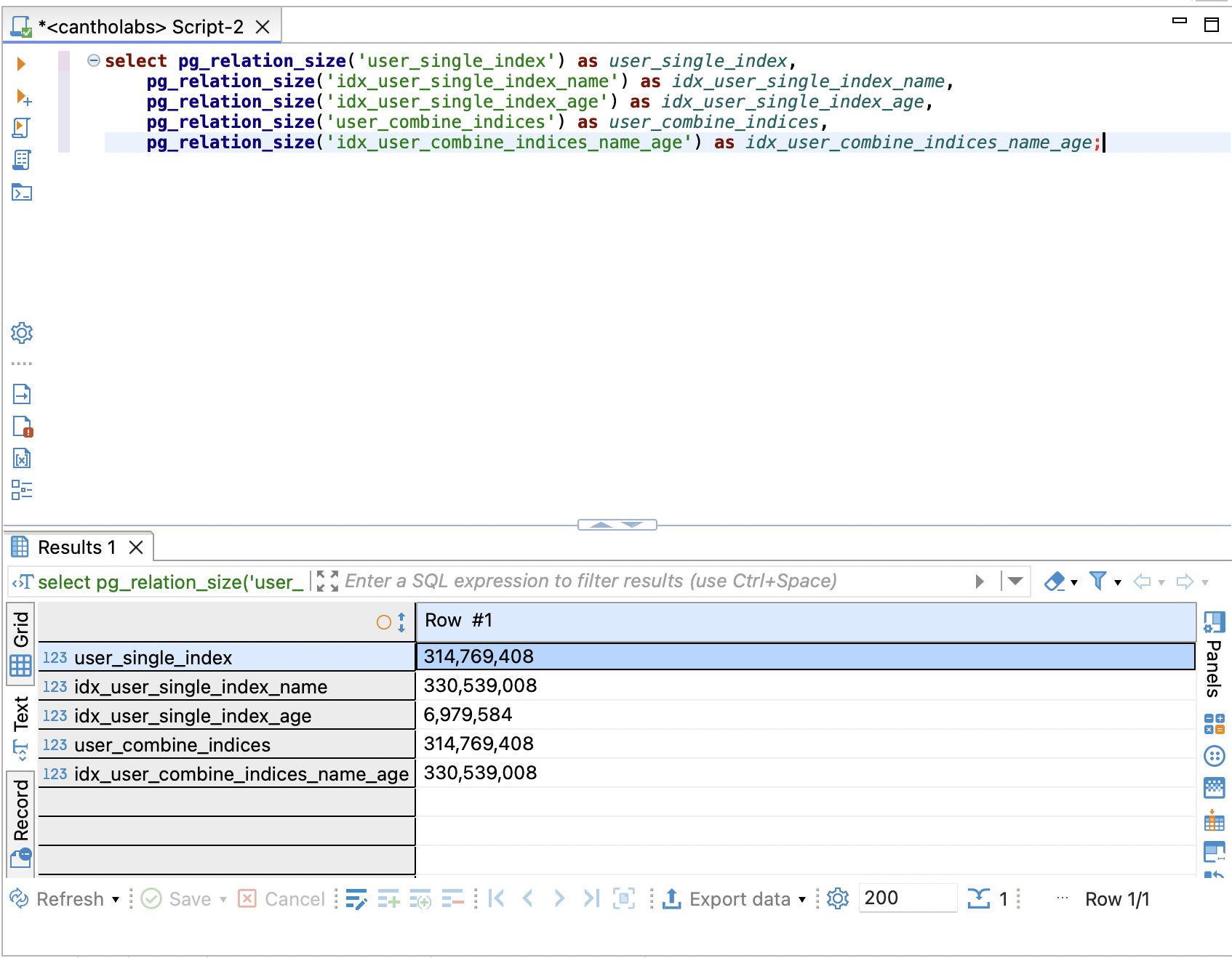
SELECT pg_relation_size('user_single_index') AS user_single_index,
	pg_relation_size('idx_user_single_index_name') AS idx_user_single_index_name,
	pg_relation_size('idx_user_single_index_age') AS idx_user_single_index_age,
	pg_relation_size('user_combine_indices') AS user_combine_indices,
	pg_relation_size('idx_user_combine_indices_name_age') AS idx_user_combine_indices_name_age;

And you know what? The index sizes are nearly equal to the size of the table. Let’s imagine what happens if you have many indices on a table that is 500GB.

Never, ever create index on updated_at (AI generated)

The standard UPDATE mechanism carries a significant performance cost, especially on tables with many indexes. A single row update requires inserting a new heap tuple, deleting the old one, and for each of the N indexes on the table, deleting the old index entry and inserting a new one. This results in a massive write amplification of 2N+1 physical writes for one logical update.

To mitigate this, PostgreSQL employs a critical optimization called Heap-Only Tuples (HOT). A HOT update is possible when an UPDATE operation does not modify any columns that are part of any index on the table. Under these conditions, PostgreSQL can perform a much more efficient update:

• A new version of the tuple is created, just like a normal update.
• Crucially, this new tuple version is placed on the same data page as the old version, provided there is sufficient free space.
• Instead of updating any indexes, the system creates a redirect pointer. The t_ctid field of the old tuple version is updated to point directly to the new tuple version on the same page.  

This creates a “HOT chain” on the page. When an index scan lands on the original tuple version, the database engine follows the t_ctid chain to the current, live version. The benefit is immense: the 2N expensive index write operations are completely avoided. This transforms the performance characteristics of UPDATEs, making schema design—specifically, the choice of which columns to index—a critical factor in write performance. A common performance anti-pattern is to index a frequently updated column (e.g., a updated_at field), as doing so completely disables the HOT optimization for that table, potentially degrading UPDATE performance by an order of magnitude.

Conclusion

In this post, we have explored some tips and tricks for designing and operating database systems more effectively and easily. Use them with caution and always consider the trade-offs involved in each approach.